Home » Case study » Short circuit faults detection for VFD-driven induction motor
Short circuit faults detection for VFD-driven induction motor
Abstract
This work is the application of a Multilayer Perceptron Artificial Neural Network (MLP ANN) to detect early inter turn short-circuit faults in a three phase variable frequency drive (VFD) driven induction motor. The quantity used to analyze the problem is the stator current or, more specifically, the harmonic contend of its frequency spectrum, also called current signature. The analysis through the current signature is a non-invasive method and can be embedded in the VFD, what is a great advantage. The data sheet used to training and to validate the Artificial Neural Network is obtained using a test bench that allows to apply different levels of inter turn short-circuits in the machine. It is observed that the fault motor data sheet and healthy motor data sheet are difficult to separate due the nonlinear character, which demands a large computational effort to choose an appropriate Multilayer Perceptron topology. The Multilayer Perceptron is trained by two different algorithms (the classical error Back-Propagation - BP - and an adaptation of the newer Extreme Learning Machine - ELM) and the results are thoroughly explored. Then it is slightly compared with the results of a Self-Organized Map Artificial Neural Network obtained by using the same data sheet.
Introduction
The induction machine is consolidated as main motor force in industries. According Thomson and Fenger, in an industrialized nation the induction motor might consume, typically, among 40% and 50% of all capacity generated.
Despite the recognized robustness and reliability of this machine, it is subject to fault occurrence, many times due to installation environment conditions, inadequate applications and lack of preventive maintenance. The more common occurrences are bearing faults, stator or rotor isolation faults, open bars or crack of the rings and eccentricity fault.
Machine faults produce symptoms like unbalanced line voltage and current, increasing in torque pulsation, decreasing in the mean torque, increasing of losses, efficiency decreasing, and excessive heating. Therefore several methods of detection and diagnostic has been developed past years and new solutions keep appearing with the objective to increase the accuracy but also to simplify techniques and to decrease costs.
In industries the cost of an unscheduled production downtime is too high; hence they invest increasingly to improve their maintenance programs. Faults like open rotor bars, eccentricity and bearing faults take time to evolve and put the motor out of operation. In this context, the constant online monitoring is important to early fault detection in a way to have time to program a maintenance order and save the machine.
The stator winding inter-turn short-circuit (SWITSC) takes a short time to evolve and to condemn the motor. Thomson and Fenger tested low voltage three-phase induction machines from early SWITSC until complete failure and found that exist a time of a few minutes to occur the fault evolution. This time is probably not enough to avoid unscheduled production downtime. But the early detection makes possible to repair the machine by rewinding it or, in large machines, removing short-circuited coils and the early operation stopping avoids electrical arcs due short-circuit and then offers an additional protection to areas where there are explosion risks. Moreover, after the severe fault, the ferromagnetic core is damaged and the machine becomes probably irreparable.
It has become more and more common the use of VFD to drive induction motors. That gives more versatility to the VFD of machines because it allows application with varying rotation speed. The high current in the motor due to fault also affects the VFD integrity and an early detection means an additional protection. Moreover, once this electronics is already being in use, could be advantageous have detection systems previously embedded in it. Past years the developing of several computational intelligence techniques added new possibilities to fault detection and diagnosis systems, most of them potentially suitable to be embedded in electronic variable frequency drives. Examples include Artificial Neural Network, fuzzy systems, genetic algorithms, among others.
Despite the spread of variable frequency drive driven machines, most of researches uses line-driven VFD machine. Using variable frequency drive-driven motor, Kowalski and Wolkiewicz analyze the spectrum of instantaneous Park power and torque signals to diagnosis early SWITSC and broken rotor bars. The same authors in use neural networks to diagnosis SWITSC with 80% of accuracy. Coelho and Medeiros in try to map the SWITSC fault using self-organized map and classify the motor.
According Nandi et al, isolation fault represents from 30% to 40% of all kinds of faults reported in induction motors. This significant amount justifies the detailed investigation of the problem. In this work is investigated the motor current signature analysis (MCSA) together with the potential of a single hidden-layer feed-forward neural network (SLFN) classifier as a tool of in SWITSC detection to variable frequency drive-driven three-phase induction machine. Two algorithms were used to training the neural network: the error back-propagation (BP), which is the classical one, and the ELM, which is a more recent algorithm. The data sheets were obtained by an experimental test bench where different level of SWITSC can be applied.
Stator Winding Inter-Turn Short-Circuit Overview
Isolation systems are submitted to several kinds of efforts that might cause a failure. Due the use of variable frequency drives to drive electrical motors with a typically frequency switching of about 10 kHz, occur voltage peaks such that increases considerably the machine isolation stress. As result, the driven variable frequency drive motor stress might be until ten times higher than line driven machines.
The failure process is usually initialized as a turn-to-turn high impedance fault (order of kΩ) in the same phase, between phases or phase-to-ground. The fault current can reaches two times the rotor blocked current, which causes high localized heating and makes the fault quickly spreads. If the incipient fault was detected it is possible reutilize the machine after repairs, but if the fault evolves might possibly causes an irreparable damage to the machine core.
Different methods have been used in many researches to detect stator inter-turn short-circuit. Ballal et al use the symmetric components theory to do the detection. This technique consists in using an expression to separate the currents in positive, negative and zero sequences. They analyze a graphic that the positive and negative sequences describe a circle with opposite spinning direction. The detection is done by a measure of the deformation caused in the graphics by the fault.
Boqiang et al use as characteristic to detection the negative impedance sequence, which is defined as the negative sequence value of the voltage component divided by the negative sequence current component. In experimental tests they realized that there is an oscillation of the impedance value with time and it is necessary a low-pass filter to guarantee the technic reliability.
Considering the MCSA, Joksimovic and Penman show that there are no novel components in stator motor current frequency spectrum due to the isolation fault. In fact it was observed that just occur an increase of the existents components. Stavrou et al search the current frequency spectrum for the variation in frequencies as function of number of poles, slots and slip, that is, specific constructive features.
Penman et al develop an equation (1) to calculate which harmonic components in the axial leakage flux waveform are functions of the SWITSC and propose a method to detect fault by monitoring those components.
According Das et al unbalanced supply voltage might produce current signature which look apparently identical to stator winding inter-turn fault cases. They propose a method to separate these two signatures. Their method is based in the Extend Park's Vector Approach (EPVA) and combined with signal processing tool as Fast Fourier Transform (FFT), Discrete Wavelet Transform (DWT) and Power Spectral Density (PSD) to make the discrimination.
Thomson and Fenger expand the concept of the leakage flux to stator currents, once the flux inside the machine also crosses the stator windings. They do an experimental analysis in low voltage motors to verify which frequencies are function just of the short-circuit and no other conditions as unbalanced phases, misalignment of the shaft, broken rotor bars, bearing faults, etc. The components using equation (1) as function only of short-circuit are fst1 when k=1, n=3 and k=1, n=5; to an unload motor (s≈0) with 2 pair of poles, these harmonics would be 2.5f1 and 3.5f1.
Also using MCSA, Gazzana et al create a system to early detection and diagnosis rotor broken bars, air-gap eccentricities and SWITSC in induction motors. To SWITSC the equation (1) is used with k=1, n=7 and the Welch‟s method is used to obtain the frequency spectrum. The choice of a high order spatial component in the spectrum is because the low order eccentricity components are coincident with short-circuit components.
Based on stator currents Hyun et al create neural models to simulate the state of one induction motor without any faults, one with isolation fault and other with bearing fault. The models are put in parallel with the system and the real output are constantly compared with the neural models outputs. A Bayesian network evaluates the model residues and detects the isolation or bearing fault.
Bouzid et al use a neural network to locate the phase where the short-circuit is. It is chosen as fault feature the phase shift between the three phase voltages and currents. The detection is made by a Multilayer Perceptron NN with 3 outputs, each one referent to one phase. If that neuron was active it means a fault in that phase. They validate the method using two induction motors and conclude it is an efficient method and once a NN was trained to one motor it can be used to other identical machines.
Das et al process the line current signal recorded from motor terminals through a Parks transformation followed by Continuous Wavelet Transformation and uses a Support Vector Machine (SVM) to classify the extracted features. From the 18 test cases used for prediction, a total of 16 fault cases were correctly identified by the proper configured SVM.
Among all possible methods to fault detection, current signature has a great potential because it is non-invasive; does not require installation of sensor in the machine; does not require be adapted to classified areas (because it can be installed at the panel, far from potential explosive mixtures); presents high capacity of remote monitoring reducing the maintenance men exposition to risks; can be applied to any machine, with no power restriction; presents sensitivity to mechanical machine faults, stator electric faults and feed problems; among others. To these advantages it can be added, to variable frequency drive-driven motors, the possibility of embedded the detection system in the own variable frequency drive, especially if a computational intelligence technique was used.
This work presents a Multilayer Perceptron Artificial Neural Network to classification of SWITSC. The equation (1) developed by the Penman's theory and expanded by Thompson is initially used for feature extraction to the fault detection.
Multilayer Perceptron Artificial Neural Network in a Nutshell
The Artificial Neural Networks appeared as mathematics tool based on the human brain biological model. Simplified models based are usually designed to specific problems solutions like classification, pattern matching, pattern completion, optimization, control, function approximation and data mining.
It was proved that an Multilayer Perceptron Artificial Neural Network with one hidden layer can approximate any continuous function with a determined precision since it has neurons enough. In classification they are recommended for applications in which there is an unknown non-linear relation between input and output data sheet, even for complex non-linear multi-variable problems. They are capable to learn this relationship by data presentation and then generalize the knowledge and classify new data.

Fig. 1 Generic Single-Hidden Layer Feedforward Neural Network
In Fig. 1 is shown a generic architecture of a SLFN. First there is the input vector, that's fully connected with the hidden layer by the weights wij just like the synapses that connect biological neurons. The hidden layer uses non-linear function to make a transformation in data space and produces a linear-separable data space. The hidden-layer output is the input to the output layer, where the classification is done.
The Multilayer Perceptron Artificial Neural Network trained by BP algorithm (MLP/BP) is probably the most studied and classical neural model, especially in classification applications, but even nowadays, a user soon becomes aware of the difficulties in finding an optimal architecture for real-world applications. An architecture that is too small will not be able to learn from data properly. Otherwise, an architecture having too many hidden neurons are prone to fit too much of the noise on the training data.
The many parameters that need to be adjust by heuristic or more commonly by attempt and error demands much time and effort to design a proper Multilayer Perceptron, also the time wasted with the BP training is usually elevated. That led many researchers to look for a new algorithm that overcome the classical.
A new learning algorithm for SLFNs named ELM and has become the aim of many studies. The two great advantages of the ELM are easy neural network design, which has practically no parameters to adjust and the training algorithm that computes extremely fast.
Experimental Data Acquisition
To collect the data sheet needed to training the Artificial Neural Networks, an induction motor was rewound by a specialized company. The motor is a WEG with rated values: 0.75kW (1.0 CV) 60Hz, 220/380V, 3.02/1.75A, n=1720rpm, efficiency: 79.5%, F.P.=0.82. Originally each phase is composed by 2 groups of 3 concentric windings, each one with 58 coils. After rewinding, coil derivations of one group of each one of the three phases were let outside the motor frame the way to allow apply SWITSC. In Figure 2 (b) it is shown the derivations details. A Gozuk VFD was used to drive the motor and a Foucault‟s brake - Figure 2 (a) - was used to apply load. The data was acquired by a data acquisition system Agilent U2352 with 16 bits of resolution, passing through a 1 kHz analog filter and a signal amplifier; that implies the band used to work is limited to 500 Hz.

Fig. 2 (a) Induction motor extern derivations details and bornes and (b) Coupling Motor-Load (Foulcault’s brake).
The three phase current signals are measured by hall sensors and collected with a frequency of sample of 10 kHz during 10 seconds. That creates a data sheet of 100,000 samples to each phase.
The motor is delta connected. To the acquisition the VFD is set to seven different values: 30 Hz, 35 Hz, …, 60 Hz. Furthermore, three load conditions are considered: unload motor, 50% rated load motor and 100% rated load motor.
To cover a considerable range of the SWITSC fault it was defined two kinds of short circuit: high impedance (HI) and low impedance (LI). The first one emulates the incipient SWITSC and the second one emulates a more severe fault. In the Figure 3 it is shown the simplified scheme of each kind of fault. In Figure 3 (a) the resistor creates a parallel way with high impedance to the current flows, similar to the first stage of short-circuit. In Figure 3 (b) the resistor limits at nominal the current that flows by electromagnetic induction in group 2, but the impedance between groups 1 and 3 is low.
One of the three phases is chosen to be short-circuited to the data acquisition tests. Three crescent levels of inter-turn short- circuits are applied both in HI and LI. Represented as the percentage of the total number of stator windings in that phase, the levels are approximately 1.41%, 4.81% and 9.26%. In the following text the HI fault might be referred as HI1, HI2 and HI3 that means HI with 1.41%, with 4.81% and with 9.26% of short circuited windings respectively. The same is valid to LI fault.

Fig. 3 Emulation scheme of: a) high impedance and b) low impedance.
Data sheets
Two mainly data sheets created are the healthy and the fault data sheets, but is important to emphasize that the fault condition can be subdivided in HI fault and LI fault. The HI and LI can once more be subdivided according the level of inter-turn short circuit (HI1, HI2, HI3, LI1, LI2, LI3).
The normal condition and each one of the subdivided fault (HI1, HI2, HI3, LI1, LI2, LI3) contains 100,000 time domain samples to each phase. The spectrum in frequency domain is obtained by the Fast Fourrier Transform (FFT). From the each spectrum some multiples are chosen as neural networks input attributes.
Due there is redundant information given by the two phases directly connect with the short circuit, one of them is unnecessary and can be excluded. Then the phase B current is not used in the data sheets which gives a total amount of samples equal to 378 (2 classes x 2 currents x 7 frequencies x 3 loads x 2 kinds of fault x 3 levels of fault). The normal conditions data sheet has 42 samples (2 currents x 7 frequencies x 3 loads), and the fault condition has 336 samples, which 168 are HI and 168 LI.
To a practical implementation of the classifier, only one sensor in anyone of the three phases would be necessary to detection. That is possible because the Artificial Neural Network is trained with the characteristics of the phase directly connected to the short-circuit as well as with the phase not directly connected to it.
Attributes Selection
The equation (1) is used to make a pre-selection of the harmonics used as Artificial Neural Network attributes. Considering the s=0 and known that p=2, the spectrums when k=1 and n=1,2,3,4,5, ... obtained from equation (1) are: 0.5f1, 1f1, 1.5f1, 2f1, 2.5f1, 3f1, …. But the slip will never be zero; it depends on the load and also of the VFD frequency. So an algorithm is used to get the amplitude of approximated harmonics: those harmonics are used as a central point and a search for the maximum amplitude value around each one of them is done. The range to the search is ±s. Due the band limit of 500 Hz, it is done until 8th harmonic, which gives 16 pre-selected parameters.
Summarizing, the pre-selected attribute vector contain 16 values that are the approximated spectrum given by equation (1). To reduce this number, it was done a statistic analysis of the variance of the pre-selected attributes considering all the conditions used (load, frequencies, kind of faults, level of faults). The attributes are reduced to 0.5f; 1f; 1.5f; 2f; 3f; 5f; 7f, but it was not the final ones. It was included also 2.5f, 3.5f because these are the approximated harmonics to a 4 pole motor according that gives information about short-circuit, but after testing each component relevancy of these harmonics to the Artificial Neural Network, the final attributes chosen were 0,5f; 1,5f; 2,5f; 3f; 5f; 7f.

Fig. 4 Variance analysis to attributes selection.
Results
During the training of the Artificial Neural Networks 90% of data samples were used. The 10% remained composed the validation data sheet. However, the training data sheet was equally divided to each class in a way to avoid tendentious classification. Consequently, due the healthy data sheet has 42 samples and the faulty condition has 336 samples, great part of the faulty data sheet are not used during the training, so these data are added to validation data sheet.
There are no formulas to select the BP parameters, so all the parameters used were selected after several attempts. At the end the hidden-layer was set to 5 neurons. The learning rate used decreases exponentially with the number of epochs until a final value. Also it was used a momentum term of 0.8. It was implemented the early stop, that uses a test data sheet to stop the training when the generalizing error is growing. Thus the data sheets has to be divided to training, testing and validation. Respectively, they were set to 70%, 20% and 10% of the total. To the ELM, the only parameter to be adjusted is the number of hidden-layers that was set to 20 after many experiments.
In Both Artificial Neural Networks the activation functions are hyperbolic tangents and the data sheets were normalized by two ways: i) removing the average and dividing by variance and ii) by adjusting the values between -1 and +1.
To evaluate a classifier performance it is commonly used the classification rate, that is given by the numbers of vectors correctly classified divided by the total numbers of all classes vectors. Many researchers usually evaluate the validation data sheet only, i.e. the generalization capability with new data. But many samples are used during the training and then the classification rate found to training data sheet is considered important.
Moreover, using simple global classification rate do not give an evaluation about individual performance of each class classification, then is common to complement the performance evaluation by the use of a confusion matrix CM. The diagonal of the CM has the classification rate to each class.
The Artificial Neural Networks and its algorithms are programed using the software MATLAB version 7.11. In Table 1 is shown the average results found after 50 trainings and its standard deviation. Some abbreviations are used: CR for classification rate; the subscripts TR, TS and VAL refer to training, test and validation data sheets; respectively; σ for standard deviation; Nh for the number of hidden-neurons; Nw for the total number of weights.
To attest the non-linear separability of the data sheets it was included a test with the simple perceptron which is a linear neural classifier. In Table 2 is shown the Confusion Matrix Average CM.
Table 1. Average results of the Artificial Neural Networks.
The linear classifier Perceptron hits on average about 60% of the training data sheet. It means the Perceptron has no capability of mapping the data sheet. It also presents poor generalization capability. Looking to Multilayer Perceptron results with BP and ELM it is realizable that the classification to this problem is a hard task even using non-linear classifiers: on average about 65% of the new data are correctly classified both to MLP/BP as to MLP/ELM. The number of weights in MLP/ELM is almost 4 times greater than the MLP/BP, which is an important feature when one thinks in to embed the Artificial Neural Network in micro-processors with limited memory capacity.
Table 2. Confusion Matrices Average.
The MLP/BP present more equally classification, it is possible to see in CMTR that about 75% of faulty data were correctly classified on average, and about 80% of the healthy were correctly classified. That is a discrepancy of about 5% whereas in the MLP/ELM this discrepancy is about 10%.
Table 3. Percentages of correctly classification to each level of short-circuit.
The faulty data sheet is composed by 6 sub-divisions of faults, as early mentioned, named here as HI1, HI2, HI3, LI1, LI2, LI3. Table 3 shows the average of the correctly classification to each level of fault to training and test data sheet. It is possible to see that the more coils are short-circuited, the faults are more correctly classified.
Average results are used to evaluate the general behavior of the designed neural networks, but in the real implementation one Artificial Neural Network must be chosen. Then one Artificial Neural Network trained by back-propagation and other trained by ELM were chosen to be pruning and then used to show the final results.
The choice of the specifics Artificial Neural Networks take in consideration the classification rate of validation and training data sheets, but it was observed mainly the CR to each class. The priority was to choose an Artificial Neural Network that correctly classified all the healthy conditions in the validation data sheets. That choice aims to avoid false positives in an online constant monitoring.
Table 4. Results to specifics Artificial Neural Networks.
In Table 4 it is shown that the specific MLP /BP reaches better classification both to training data sheet as to validation data sheet. Moreover, after pruning the MLP/BP was able to improve its generalization capacity. The MLP/ELM was not able to be appropriated pruned by the CAPE method.
In the same data sheet used in this work was used in a Self-Organized Map Artificial Neural Network. There are differences in attributes used, and in data sheets normalization. The final result presented by gives a global CR of 87.5%. However, the CR to healthy data sheet is 52%, whereas the CR to faulty data sheet is 94.5%. That result means the most data are classified as faulty which is larger than the healthy data sheet. In an online constant monitoring it also probably means that there is a high probability of false positives occurrence.
Conclusions
The problem of early fault detection in driven-variable frequency drive induction motor is a subject that is far to be completely solved. The investigation with real data sheets reveals difficulties in separating the faulty data sheets from the healthy ones, which reinforces the importance of constant on-line monitoring. The use of variable frequency drive adds the possibility of to embed the system directly in the equipment, which means more protection to the variable frequency drive besides all the discussed benefits of early fault detection to the machine and to industries. The great advantages of this non-invasive detection system make its improvement a task with great potential; one possibility involves the choice of relevant spectrums as parameters to training the classificator which is not an ended issue and is directly related with the classifier accuracy.
The two algorithms used to training the classifier showed similar results, but the ELM computes much faster and is much easier designed, although the MLP/ELM needed four times more neurons in the hidden- layer to do so. The pruning method was capable to improve the generalization in MLP/BP through the removing of connections, but the MLP/ELM was not able to be pruning by the method used.
This work is the application of a Multilayer Perceptron Artificial Neural Network (MLP ANN) to detect early inter turn short-circuit faults in a three phase variable frequency drive (VFD) driven induction motor. The quantity used to analyze the problem is the stator current or, more specifically, the harmonic contend of its frequency spectrum, also called current signature. The analysis through the current signature is a non-invasive method and can be embedded in the VFD, what is a great advantage. The data sheet used to training and to validate the Artificial Neural Network is obtained using a test bench that allows to apply different levels of inter turn short-circuits in the machine. It is observed that the fault motor data sheet and healthy motor data sheet are difficult to separate due the nonlinear character, which demands a large computational effort to choose an appropriate Multilayer Perceptron topology. The Multilayer Perceptron is trained by two different algorithms (the classical error Back-Propagation - BP - and an adaptation of the newer Extreme Learning Machine - ELM) and the results are thoroughly explored. Then it is slightly compared with the results of a Self-Organized Map Artificial Neural Network obtained by using the same data sheet.
Introduction
The induction machine is consolidated as main motor force in industries. According Thomson and Fenger, in an industrialized nation the induction motor might consume, typically, among 40% and 50% of all capacity generated.
Despite the recognized robustness and reliability of this machine, it is subject to fault occurrence, many times due to installation environment conditions, inadequate applications and lack of preventive maintenance. The more common occurrences are bearing faults, stator or rotor isolation faults, open bars or crack of the rings and eccentricity fault.
Machine faults produce symptoms like unbalanced line voltage and current, increasing in torque pulsation, decreasing in the mean torque, increasing of losses, efficiency decreasing, and excessive heating. Therefore several methods of detection and diagnostic has been developed past years and new solutions keep appearing with the objective to increase the accuracy but also to simplify techniques and to decrease costs.
In industries the cost of an unscheduled production downtime is too high; hence they invest increasingly to improve their maintenance programs. Faults like open rotor bars, eccentricity and bearing faults take time to evolve and put the motor out of operation. In this context, the constant online monitoring is important to early fault detection in a way to have time to program a maintenance order and save the machine.
The stator winding inter-turn short-circuit (SWITSC) takes a short time to evolve and to condemn the motor. Thomson and Fenger tested low voltage three-phase induction machines from early SWITSC until complete failure and found that exist a time of a few minutes to occur the fault evolution. This time is probably not enough to avoid unscheduled production downtime. But the early detection makes possible to repair the machine by rewinding it or, in large machines, removing short-circuited coils and the early operation stopping avoids electrical arcs due short-circuit and then offers an additional protection to areas where there are explosion risks. Moreover, after the severe fault, the ferromagnetic core is damaged and the machine becomes probably irreparable.
It has become more and more common the use of VFD to drive induction motors. That gives more versatility to the VFD of machines because it allows application with varying rotation speed. The high current in the motor due to fault also affects the VFD integrity and an early detection means an additional protection. Moreover, once this electronics is already being in use, could be advantageous have detection systems previously embedded in it. Past years the developing of several computational intelligence techniques added new possibilities to fault detection and diagnosis systems, most of them potentially suitable to be embedded in electronic variable frequency drives. Examples include Artificial Neural Network, fuzzy systems, genetic algorithms, among others.
Despite the spread of variable frequency drive driven machines, most of researches uses line-driven VFD machine. Using variable frequency drive-driven motor, Kowalski and Wolkiewicz analyze the spectrum of instantaneous Park power and torque signals to diagnosis early SWITSC and broken rotor bars. The same authors in use neural networks to diagnosis SWITSC with 80% of accuracy. Coelho and Medeiros in try to map the SWITSC fault using self-organized map and classify the motor.
According Nandi et al, isolation fault represents from 30% to 40% of all kinds of faults reported in induction motors. This significant amount justifies the detailed investigation of the problem. In this work is investigated the motor current signature analysis (MCSA) together with the potential of a single hidden-layer feed-forward neural network (SLFN) classifier as a tool of in SWITSC detection to variable frequency drive-driven three-phase induction machine. Two algorithms were used to training the neural network: the error back-propagation (BP), which is the classical one, and the ELM, which is a more recent algorithm. The data sheets were obtained by an experimental test bench where different level of SWITSC can be applied.
Stator Winding Inter-Turn Short-Circuit Overview
Isolation systems are submitted to several kinds of efforts that might cause a failure. Due the use of variable frequency drives to drive electrical motors with a typically frequency switching of about 10 kHz, occur voltage peaks such that increases considerably the machine isolation stress. As result, the driven variable frequency drive motor stress might be until ten times higher than line driven machines.
The failure process is usually initialized as a turn-to-turn high impedance fault (order of kΩ) in the same phase, between phases or phase-to-ground. The fault current can reaches two times the rotor blocked current, which causes high localized heating and makes the fault quickly spreads. If the incipient fault was detected it is possible reutilize the machine after repairs, but if the fault evolves might possibly causes an irreparable damage to the machine core.
Different methods have been used in many researches to detect stator inter-turn short-circuit. Ballal et al use the symmetric components theory to do the detection. This technique consists in using an expression to separate the currents in positive, negative and zero sequences. They analyze a graphic that the positive and negative sequences describe a circle with opposite spinning direction. The detection is done by a measure of the deformation caused in the graphics by the fault.
Boqiang et al use as characteristic to detection the negative impedance sequence, which is defined as the negative sequence value of the voltage component divided by the negative sequence current component. In experimental tests they realized that there is an oscillation of the impedance value with time and it is necessary a low-pass filter to guarantee the technic reliability.
Considering the MCSA, Joksimovic and Penman show that there are no novel components in stator motor current frequency spectrum due to the isolation fault. In fact it was observed that just occur an increase of the existents components. Stavrou et al search the current frequency spectrum for the variation in frequencies as function of number of poles, slots and slip, that is, specific constructive features.
Penman et al develop an equation (1) to calculate which harmonic components in the axial leakage flux waveform are functions of the SWITSC and propose a method to detect fault by monitoring those components.
1) fst = {k ± n(1-s)/p}f1The fst is inter-turn short-circuit function components, k=1, 3, 5..., means the temporal harmonics order, n= 1, 2, 3..., means the spatial harmonic order, s is the slip, p is the pair of poles, f1 is the power supply fundamental frequency. Several kinds of faults affect the current spectrum and some harmonics are affected by more than one abnormal condition, so one must be careful to choose the correct frequencies that will be used to indicate the problem.
According Das et al unbalanced supply voltage might produce current signature which look apparently identical to stator winding inter-turn fault cases. They propose a method to separate these two signatures. Their method is based in the Extend Park's Vector Approach (EPVA) and combined with signal processing tool as Fast Fourier Transform (FFT), Discrete Wavelet Transform (DWT) and Power Spectral Density (PSD) to make the discrimination.
Thomson and Fenger expand the concept of the leakage flux to stator currents, once the flux inside the machine also crosses the stator windings. They do an experimental analysis in low voltage motors to verify which frequencies are function just of the short-circuit and no other conditions as unbalanced phases, misalignment of the shaft, broken rotor bars, bearing faults, etc. The components using equation (1) as function only of short-circuit are fst1 when k=1, n=3 and k=1, n=5; to an unload motor (s≈0) with 2 pair of poles, these harmonics would be 2.5f1 and 3.5f1.
Also using MCSA, Gazzana et al create a system to early detection and diagnosis rotor broken bars, air-gap eccentricities and SWITSC in induction motors. To SWITSC the equation (1) is used with k=1, n=7 and the Welch‟s method is used to obtain the frequency spectrum. The choice of a high order spatial component in the spectrum is because the low order eccentricity components are coincident with short-circuit components.
Based on stator currents Hyun et al create neural models to simulate the state of one induction motor without any faults, one with isolation fault and other with bearing fault. The models are put in parallel with the system and the real output are constantly compared with the neural models outputs. A Bayesian network evaluates the model residues and detects the isolation or bearing fault.
Bouzid et al use a neural network to locate the phase where the short-circuit is. It is chosen as fault feature the phase shift between the three phase voltages and currents. The detection is made by a Multilayer Perceptron NN with 3 outputs, each one referent to one phase. If that neuron was active it means a fault in that phase. They validate the method using two induction motors and conclude it is an efficient method and once a NN was trained to one motor it can be used to other identical machines.
Das et al process the line current signal recorded from motor terminals through a Parks transformation followed by Continuous Wavelet Transformation and uses a Support Vector Machine (SVM) to classify the extracted features. From the 18 test cases used for prediction, a total of 16 fault cases were correctly identified by the proper configured SVM.
Among all possible methods to fault detection, current signature has a great potential because it is non-invasive; does not require installation of sensor in the machine; does not require be adapted to classified areas (because it can be installed at the panel, far from potential explosive mixtures); presents high capacity of remote monitoring reducing the maintenance men exposition to risks; can be applied to any machine, with no power restriction; presents sensitivity to mechanical machine faults, stator electric faults and feed problems; among others. To these advantages it can be added, to variable frequency drive-driven motors, the possibility of embedded the detection system in the own variable frequency drive, especially if a computational intelligence technique was used.
This work presents a Multilayer Perceptron Artificial Neural Network to classification of SWITSC. The equation (1) developed by the Penman's theory and expanded by Thompson is initially used for feature extraction to the fault detection.
Multilayer Perceptron Artificial Neural Network in a Nutshell
The Artificial Neural Networks appeared as mathematics tool based on the human brain biological model. Simplified models based are usually designed to specific problems solutions like classification, pattern matching, pattern completion, optimization, control, function approximation and data mining.
It was proved that an Multilayer Perceptron Artificial Neural Network with one hidden layer can approximate any continuous function with a determined precision since it has neurons enough. In classification they are recommended for applications in which there is an unknown non-linear relation between input and output data sheet, even for complex non-linear multi-variable problems. They are capable to learn this relationship by data presentation and then generalize the knowledge and classify new data.
Fig. 1 Generic Single-Hidden Layer Feedforward Neural Network
In Fig. 1 is shown a generic architecture of a SLFN. First there is the input vector, that's fully connected with the hidden layer by the weights wij just like the synapses that connect biological neurons. The hidden layer uses non-linear function to make a transformation in data space and produces a linear-separable data space. The hidden-layer output is the input to the output layer, where the classification is done.
The Multilayer Perceptron Artificial Neural Network trained by BP algorithm (MLP/BP) is probably the most studied and classical neural model, especially in classification applications, but even nowadays, a user soon becomes aware of the difficulties in finding an optimal architecture for real-world applications. An architecture that is too small will not be able to learn from data properly. Otherwise, an architecture having too many hidden neurons are prone to fit too much of the noise on the training data.
The many parameters that need to be adjust by heuristic or more commonly by attempt and error demands much time and effort to design a proper Multilayer Perceptron, also the time wasted with the BP training is usually elevated. That led many researchers to look for a new algorithm that overcome the classical.
A new learning algorithm for SLFNs named ELM and has become the aim of many studies. The two great advantages of the ELM are easy neural network design, which has practically no parameters to adjust and the training algorithm that computes extremely fast.
Experimental Data Acquisition
To collect the data sheet needed to training the Artificial Neural Networks, an induction motor was rewound by a specialized company. The motor is a WEG with rated values: 0.75kW (1.0 CV) 60Hz, 220/380V, 3.02/1.75A, n=1720rpm, efficiency: 79.5%, F.P.=0.82. Originally each phase is composed by 2 groups of 3 concentric windings, each one with 58 coils. After rewinding, coil derivations of one group of each one of the three phases were let outside the motor frame the way to allow apply SWITSC. In Figure 2 (b) it is shown the derivations details. A Gozuk VFD was used to drive the motor and a Foucault‟s brake - Figure 2 (a) - was used to apply load. The data was acquired by a data acquisition system Agilent U2352 with 16 bits of resolution, passing through a 1 kHz analog filter and a signal amplifier; that implies the band used to work is limited to 500 Hz.
Fig. 2 (a) Induction motor extern derivations details and bornes and (b) Coupling Motor-Load (Foulcault’s brake).
The three phase current signals are measured by hall sensors and collected with a frequency of sample of 10 kHz during 10 seconds. That creates a data sheet of 100,000 samples to each phase.
The motor is delta connected. To the acquisition the VFD is set to seven different values: 30 Hz, 35 Hz, …, 60 Hz. Furthermore, three load conditions are considered: unload motor, 50% rated load motor and 100% rated load motor.
To cover a considerable range of the SWITSC fault it was defined two kinds of short circuit: high impedance (HI) and low impedance (LI). The first one emulates the incipient SWITSC and the second one emulates a more severe fault. In the Figure 3 it is shown the simplified scheme of each kind of fault. In Figure 3 (a) the resistor creates a parallel way with high impedance to the current flows, similar to the first stage of short-circuit. In Figure 3 (b) the resistor limits at nominal the current that flows by electromagnetic induction in group 2, but the impedance between groups 1 and 3 is low.
One of the three phases is chosen to be short-circuited to the data acquisition tests. Three crescent levels of inter-turn short- circuits are applied both in HI and LI. Represented as the percentage of the total number of stator windings in that phase, the levels are approximately 1.41%, 4.81% and 9.26%. In the following text the HI fault might be referred as HI1, HI2 and HI3 that means HI with 1.41%, with 4.81% and with 9.26% of short circuited windings respectively. The same is valid to LI fault.
Fig. 3 Emulation scheme of: a) high impedance and b) low impedance.
Data sheets
Two mainly data sheets created are the healthy and the fault data sheets, but is important to emphasize that the fault condition can be subdivided in HI fault and LI fault. The HI and LI can once more be subdivided according the level of inter-turn short circuit (HI1, HI2, HI3, LI1, LI2, LI3).
The normal condition and each one of the subdivided fault (HI1, HI2, HI3, LI1, LI2, LI3) contains 100,000 time domain samples to each phase. The spectrum in frequency domain is obtained by the Fast Fourrier Transform (FFT). From the each spectrum some multiples are chosen as neural networks input attributes.
Due there is redundant information given by the two phases directly connect with the short circuit, one of them is unnecessary and can be excluded. Then the phase B current is not used in the data sheets which gives a total amount of samples equal to 378 (2 classes x 2 currents x 7 frequencies x 3 loads x 2 kinds of fault x 3 levels of fault). The normal conditions data sheet has 42 samples (2 currents x 7 frequencies x 3 loads), and the fault condition has 336 samples, which 168 are HI and 168 LI.
To a practical implementation of the classifier, only one sensor in anyone of the three phases would be necessary to detection. That is possible because the Artificial Neural Network is trained with the characteristics of the phase directly connected to the short-circuit as well as with the phase not directly connected to it.
Attributes Selection
The equation (1) is used to make a pre-selection of the harmonics used as Artificial Neural Network attributes. Considering the s=0 and known that p=2, the spectrums when k=1 and n=1,2,3,4,5, ... obtained from equation (1) are: 0.5f1, 1f1, 1.5f1, 2f1, 2.5f1, 3f1, …. But the slip will never be zero; it depends on the load and also of the VFD frequency. So an algorithm is used to get the amplitude of approximated harmonics: those harmonics are used as a central point and a search for the maximum amplitude value around each one of them is done. The range to the search is ±s. Due the band limit of 500 Hz, it is done until 8th harmonic, which gives 16 pre-selected parameters.
Summarizing, the pre-selected attribute vector contain 16 values that are the approximated spectrum given by equation (1). To reduce this number, it was done a statistic analysis of the variance of the pre-selected attributes considering all the conditions used (load, frequencies, kind of faults, level of faults). The attributes are reduced to 0.5f; 1f; 1.5f; 2f; 3f; 5f; 7f, but it was not the final ones. It was included also 2.5f, 3.5f because these are the approximated harmonics to a 4 pole motor according that gives information about short-circuit, but after testing each component relevancy of these harmonics to the Artificial Neural Network, the final attributes chosen were 0,5f; 1,5f; 2,5f; 3f; 5f; 7f.
Fig. 4 Variance analysis to attributes selection.
Results
During the training of the Artificial Neural Networks 90% of data samples were used. The 10% remained composed the validation data sheet. However, the training data sheet was equally divided to each class in a way to avoid tendentious classification. Consequently, due the healthy data sheet has 42 samples and the faulty condition has 336 samples, great part of the faulty data sheet are not used during the training, so these data are added to validation data sheet.
There are no formulas to select the BP parameters, so all the parameters used were selected after several attempts. At the end the hidden-layer was set to 5 neurons. The learning rate used decreases exponentially with the number of epochs until a final value. Also it was used a momentum term of 0.8. It was implemented the early stop, that uses a test data sheet to stop the training when the generalizing error is growing. Thus the data sheets has to be divided to training, testing and validation. Respectively, they were set to 70%, 20% and 10% of the total. To the ELM, the only parameter to be adjusted is the number of hidden-layers that was set to 20 after many experiments.
In Both Artificial Neural Networks the activation functions are hyperbolic tangents and the data sheets were normalized by two ways: i) removing the average and dividing by variance and ii) by adjusting the values between -1 and +1.
To evaluate a classifier performance it is commonly used the classification rate, that is given by the numbers of vectors correctly classified divided by the total numbers of all classes vectors. Many researchers usually evaluate the validation data sheet only, i.e. the generalization capability with new data. But many samples are used during the training and then the classification rate found to training data sheet is considered important.
Moreover, using simple global classification rate do not give an evaluation about individual performance of each class classification, then is common to complement the performance evaluation by the use of a confusion matrix CM. The diagonal of the CM has the classification rate to each class.
The Artificial Neural Networks and its algorithms are programed using the software MATLAB version 7.11. In Table 1 is shown the average results found after 50 trainings and its standard deviation. Some abbreviations are used: CR for classification rate; the subscripts TR, TS and VAL refer to training, test and validation data sheets; respectively; σ for standard deviation; Nh for the number of hidden-neurons; Nw for the total number of weights.
To attest the non-linear separability of the data sheets it was included a test with the simple perceptron which is a linear neural classifier. In Table 2 is shown the Confusion Matrix Average CM.
Table 1. Average results of the Artificial Neural Networks.
|
Artificial Neural Network |
Nh |
Nw |
CRTR |
σTR |
CRTS |
σTS |
CRVAL |
σVAL |
|
Perceptron |
1 |
7 |
60.07% |
20.56 |
- |
- |
50.46% |
19.20 |
|
MLP/BP |
5 |
41 |
77.95% |
8.82 |
74.91% |
11.03 |
64.92% |
11.26 |
|
MLP/ELM |
20 |
161 |
85.48% |
3.67 |
- |
- |
65.17% |
4.80 |
The linear classifier Perceptron hits on average about 60% of the training data sheet. It means the Perceptron has no capability of mapping the data sheet. It also presents poor generalization capability. Looking to Multilayer Perceptron results with BP and ELM it is realizable that the classification to this problem is a hard task even using non-linear classifiers: on average about 65% of the new data are correctly classified both to MLP/BP as to MLP/ELM. The number of weights in MLP/ELM is almost 4 times greater than the MLP/BP, which is an important feature when one thinks in to embed the Artificial Neural Network in micro-processors with limited memory capacity.
Table 2. Confusion Matrices Average.
|
Artificial Neural Network |
CMTR (%) |
CMTS (%) |
CMVAL (%) |
|
MLP/BP |
Healthy Faulty Healthy 80.21 19.79 Faulty 24.31 75.69 |
Healthy Faulty Healthy 77.45 22.55 Faulty 27.64 72.36 |
Healthy Faulty Healthy 69.33 30.67 Faulty 35.17 64.83 |
|
MLP/ELM |
Healthy Faulty Healthy 87.84 12.16 Faulty 23.00 77.00 |
- |
Healthy Faulty Healthy 75.60 24.40 Faulty 35.01 64.99 |
The MLP/BP present more equally classification, it is possible to see in CMTR that about 75% of faulty data were correctly classified on average, and about 80% of the healthy were correctly classified. That is a discrepancy of about 5% whereas in the MLP/ELM this discrepancy is about 10%.
Table 3. Percentages of correctly classification to each level of short-circuit.
|
Artificial Neural Network - data sheet |
HI1 (%) |
HI2 (%) |
HI3 (%) |
LI1 (%) |
LI2 (%) |
LI3 (%) |
|
MLP/BP - TR |
67 |
72 |
74 |
73 |
84 |
91 |
|
MLP/ELM - TR |
70 |
75 |
77 |
75 |
80 |
92 |
|
MLP/BP - VAL |
59 |
60 |
66 |
64 |
70 |
70 |
|
MLP/ELM - VAL |
60 |
61 |
66 |
64 |
67 |
72 |
The faulty data sheet is composed by 6 sub-divisions of faults, as early mentioned, named here as HI1, HI2, HI3, LI1, LI2, LI3. Table 3 shows the average of the correctly classification to each level of fault to training and test data sheet. It is possible to see that the more coils are short-circuited, the faults are more correctly classified.
Average results are used to evaluate the general behavior of the designed neural networks, but in the real implementation one Artificial Neural Network must be chosen. Then one Artificial Neural Network trained by back-propagation and other trained by ELM were chosen to be pruning and then used to show the final results.
The choice of the specifics Artificial Neural Networks take in consideration the classification rate of validation and training data sheets, but it was observed mainly the CR to each class. The priority was to choose an Artificial Neural Network that correctly classified all the healthy conditions in the validation data sheets. That choice aims to avoid false positives in an online constant monitoring.
Table 4. Results to specifics Artificial Neural Networks.
|
MLP |
NW |
CRTR |
CRTS |
CRVAL |
CMTR (%) |
CMTS (%) |
CMVAL (%) |
|
BP |
41 |
89.7 |
81.8 |
68.5 |
H F H 94.9 5.1 F 15.3 84.7 |
H F H 81.8 18.2 F 18.2 81.8 |
H F H 100.0 0.0 F 32.1 67.9 |
|
BP/ CAPE |
34 |
87.1 |
81.8 |
70.2 |
H F H 94.9 5.1 F 20.5 79.5 |
H F H 81.8 18.2 F 18.2 81.8 |
H F H 100.0 0.0 F 39.7 69.3 |
|
ELM |
161 |
84.1 |
- |
63.8 |
H F H 90.2 9.8 F 22.0 78.0 |
|
H F H 100.0 0.0 F 36.1 63.9 |
|
ELM/ CAPE |
- |
- |
- |
- |
- |
- |
- |
In Table 4 it is shown that the specific MLP /BP reaches better classification both to training data sheet as to validation data sheet. Moreover, after pruning the MLP/BP was able to improve its generalization capacity. The MLP/ELM was not able to be appropriated pruned by the CAPE method.
In the same data sheet used in this work was used in a Self-Organized Map Artificial Neural Network. There are differences in attributes used, and in data sheets normalization. The final result presented by gives a global CR of 87.5%. However, the CR to healthy data sheet is 52%, whereas the CR to faulty data sheet is 94.5%. That result means the most data are classified as faulty which is larger than the healthy data sheet. In an online constant monitoring it also probably means that there is a high probability of false positives occurrence.
Conclusions
The problem of early fault detection in driven-variable frequency drive induction motor is a subject that is far to be completely solved. The investigation with real data sheets reveals difficulties in separating the faulty data sheets from the healthy ones, which reinforces the importance of constant on-line monitoring. The use of variable frequency drive adds the possibility of to embed the system directly in the equipment, which means more protection to the variable frequency drive besides all the discussed benefits of early fault detection to the machine and to industries. The great advantages of this non-invasive detection system make its improvement a task with great potential; one possibility involves the choice of relevant spectrums as parameters to training the classificator which is not an ended issue and is directly related with the classifier accuracy.
The two algorithms used to training the classifier showed similar results, but the ELM computes much faster and is much easier designed, although the MLP/ELM needed four times more neurons in the hidden- layer to do so. The pruning method was capable to improve the generalization in MLP/BP through the removing of connections, but the MLP/ELM was not able to be pruning by the method used.
Post a Comment:
You may also like:
Featured Articles
VFD for pumps in variable flow water ...
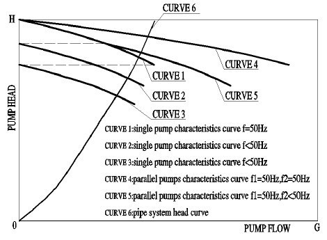 Variable flow water system has played an important role in the field of energy saving with the VFD widely used in practical ...
Variable flow water system has played an important role in the field of energy saving with the VFD widely used in practical ...Variable frequency drive energy ...
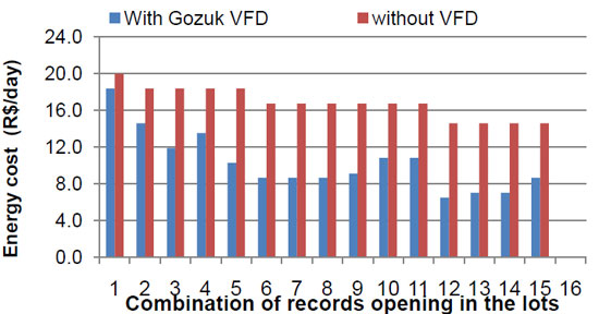 Notes that for the combinations where we had the same number of opened records, the power suffers no change, but when it is used ...
Notes that for the combinations where we had the same number of opened records, the power suffers no change, but when it is used ...Variable frequency drive on Cooling ...
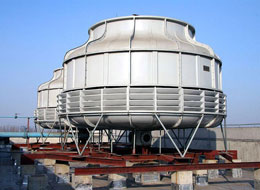 We are working on a study related to Cooling Towers. We want to decrease cooling water supply temperature going to steam ...
We are working on a study related to Cooling Towers. We want to decrease cooling water supply temperature going to steam ...VFD in China plantation irrigation ...
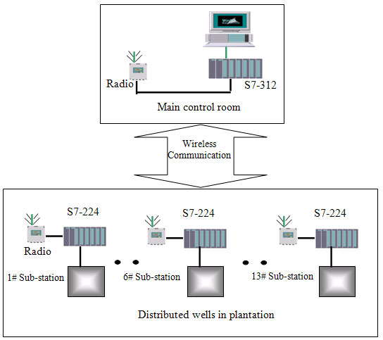 This article have a study of the wireless group control system with variable frequency drive (VFD) applied in a Chinese ...
This article have a study of the wireless group control system with variable frequency drive (VFD) applied in a Chinese ...
VFD manufacturers